Dynamic Causal Modelling of COVID-19 and Australian Projections

This webpage summarises our work to model the spread of COVID-19 pandemic. The first technical paper that introduces dynamic causal model of COVID-19 is here:

K. J. Friston, T. Parr, P. Zeidman, A. Razi, G. Flandin, J. Daunizeau, O Hulme, A. Billig, V. Litvak, R. J. Moran, C. J. Price, C. Lambert, (2020) ‘‘Dynamic causal modelling of COVID-19’’, arXiv. Link.

Here is the accompanying website which hosts open access software code, among other resources.

Dynamic causal modelling: The generative model

This figure is a schematic description of the generative model used in subsequent analyses. In brief, this compartmental model generates timeseries data based on a mean field approximation to ensemble or population dynamics. The implicit probability distributions are over four latent factors, each with four levels or states. These factors are sufficient to generate measurable outcomes; for example, the number of new cases or the proportion of people infected. The first factor is the location of an individual, who can be at home, at work, in a critical care unit (CCU) or in the morgue. The second factor is infection status; namely, susceptible to infection, infected, infectious or immune. This model assumes that there is a progression from a state of susceptibility to immunity, through a period of (pre-contagious) infection to an infectious (contagious) status. The third factor is clinical status; namely, asymptomatic, symptomatic, acute respiratory distress syndrome (ARDS) or deceased. Again, there is an assumed progression from asymptomatic to ARDS, where people with ARDS can either recover to an asymptomatic state or not. Finally, the fourth factor represents diagnostic or testing status. An individual can be untested or waiting for the results of a test that can either be positive or negative.

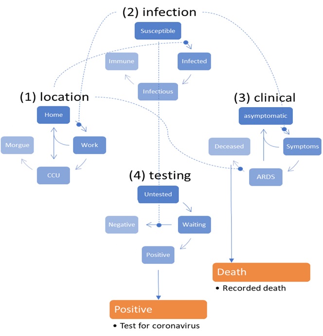With this setup, one can be in one of four places, with any infectious status, expressing symptoms or not, and having test results or not. Note that—in this construction—it is possible to be infected and yet be asymptomatic. However, the marginal distributions are not independent, by virtue of the dynamics that describe the transition among states within each factor. Crucially, the transitions within any factor depend upon the marginal distribution of other factors. For example, the probability of becoming infected, given that one is susceptible to infection, depends upon whether one is at home or at work. Similarly, the probability of developing symptoms depends upon whether one is infected or not. The probability of testing negative depends upon whether one is susceptible (or immune) to infection, and so on. Finally, to complete the circular dependency, the probability of leaving home to go to work depends upon the number of infected people in the population, mediated by social distancing. The curvilinear arrows denote a conditioning of transition probabilities on the marginal distributions over other factors. These conditional dependencies constitute the mean field approximation and enable the dynamics to be solved or integrated over time. At any point in time, the probability of being in any combination of the four states determines what would be observed at the population level. For example, the occupancy of the deceased level of the clinical factor determines the current number of people who have recorded deaths. Similarly, the occupancy of the positive level of the testing factor determines the expected number of positive cases reported. From these expectations, the expected number of new cases per day can be generated.

Dynamic causal modelling of Australian COVID-19 data

We have used this DCM to model and provide projections for new cases and fatalities in Australia in the wake of the COVID-19 spread. We used the data provided by JHU CSSE (data until 6th April). The results of this analysis are made available to showcase the modelling. They should not be taken seriously as a prediction. This is because the current cases are extremely small in number; violating the large number assumption that underwrites the likelihood model used in the DCM. Operationally, countries with cumulative deaths of less than 128 are usually excluded from the hierarchical (parametric empirical Bayesian) modelling – when testing for systematic between country differences. In one sense, if a country suffers a very small number of deaths, it can be, effectively, considered as having eluded the pandemic.

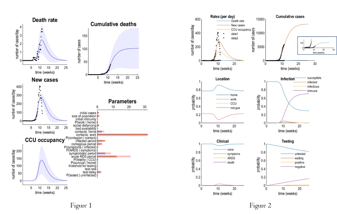Figure 1 reports predicted new deaths and cases (and CCU occupancy) for Australia. The panels on the left show the predicted outcomes as a function of weeks. The blue lines correspond to the expected trajectory, while the shaded areas are 90% Bayesian credible intervals. The black dots represent empirical data, upon which the parameter estimates are based. The lower right panel shows the parameter estimates. As in previous figures, the prior expectations are shown as pink bars over the posterior expectations (and credible intervals). The upper right panel illustrates the equivalent expectations in terms of cumulative deaths.

In Figure 2, the upper panels reproduce the expected trajectories for Australia. The expected death rate is shown in blue, new cases in red, predicted recovery rate in orange and CCU occupancy in yellow. The black dots correspond to empirical data. The (zoomed) square box on upper right panel shows the cumulative deaths otherwise not obvious. The lower four panels show the evolution of latent (ensemble) dynamics, in terms of the expected probability of being in various states. The first (location) panel shows that after about 10 weeks, there was a sufficient evidence for the onset of an episode (we are past that peak) that induced social distancing, such that the probability of being found at work falls, over a couple of weeks to negligible levels. At this time, the number of infected people increases (approx. 0.5%) with a concomitant probability of being infectious a few days later. During this time, the probability of becoming immune increases monotonically and saturates at about 20 weeks. Clinically, the probability of becoming symptomatic rises to about 0.4%, with negligible probability of developing acute respiratory distress (ARDS) and, possibly death (these probabilities are very small and cannot be seen in this graph). In terms of testing, there is a progressive increase in the number of people tested, with a concomitant decrease in those untested or waiting for their results. Under these parameters, the entire episode lasts for about 10 weeks, or less than three months.

Dynamic causal modelling of COVID-19 spread across regions

Subsequently, we combine several of these (epidemic) models to create a (pandemic) model of viral spread among regions. Our focus is on second wave of new cases that may result from loss of immunity—and the exchange of people between regions—and how mortality rates can be ameliorated under different strategic responses. In particular, we consider hard or soft social distancing strategies predicated on national (Federal) or regional (State) estimates of the prevalence of infection in the population.

K. J. Friston, T. Parr, P. Zeidman, A. Razi, G. Flandin, J. Daunizeau, O Hulme, A. Billig, V. Litvak, R. J. Moran, C. J. Price, C. Lambert, (2020) ‘‘Second waves, social distancing, and the spread of COVID-19 across America’’, arXiv. Link.

Review on Data Science and COVID-19

We have also written a comprehensive review in an attempt to systematise ongoing data science activities in this area. As well as reviewing the rapidly growing body of recent research, we survey public datasets and repositories that can be used for further work to track COVID-19 spread and mitigation strategies.

S. Latif, M. Usman, S. Manzoor, W. Iqbal, J. Qadir, G Tyson, I. Castro, A. Razi, M. N. K. Boulos, and J. Crowcroft, ‘‘Leveraging data science to combat COVID-19: A comprehensive review”, Link

Here is the accompanying website which is constantly updated with new datasets and other community resources.